for the approximation of highly singular solutions
![]()
The aim of this benchmark is to provide Maxwell problems whose solution has a strong unbounded singularity. Most of these problems can be solved alternatively by a scalar boundary value problem providing a potential for the Maxwell solution, which results into a more accurate approximation of the Maxwell solution. This fact allows us to provide reference solutions to which we will compare the results obtained by different Maxwell codes based on various methods.
We would appreciate to receive contributive results. We offer to append them to this page.
We present
1.
A list of domains (2D and 3D) where Maxwell equations are set,
2.
A list of problems to solve.
3.
A list of reference solutions for (most of) the problems we propose.
4.
Directions for use to provide a feedback.
5.
Results
- Rennes :
Finite Element Library Mélina
(posted by Monique Dauge - January 24, 2003).
- Zürich :
Software Package Concepts
(posted by Philipp Frauenfelder - September 06, 2004) - Available Again Now!
- Inria Rocquencourt :
Code Montjoie
(posted by Marc Duruflé - December 22, 2006).
We propose the computation of eigenvalues. Other computations (a source problem) will be set in (a near) future.
Aknowledgements.
We thank Jan S. Hesthaven of Brown University for useful remarks concerning this page.
![]()
![]()
The domain has straight sides and corners in (0,0), (1,0), (1,1), (-1,1), (-1,-1), (0,-1).
![]() Go back to the list of domains
Go back to the list of domains
![]()
The domain has straight sides and corners in (0,0), (1,0), (1,1), (-1,1), (-1,-1), (1,-1), (1,0).
![]() Go back to the list of domains
Go back to the list of domains
![]()
The domain has 2 straight and 2 two circular sides (of radiii 2 and 3).
Its corners are in
(2,0), (3,0), (3/sqrt(2), 3/sqrt(2)), (2/sqrt(2), 2/sqrt(2)).
![]() Go back to the list of domains
Go back to the list of domains
![]()
The domain has 3 straight and 3 two circular sides (of radii 1, 2 and 3).
Its corners are
(2,0), (3,0), (3/sqrt(2), 3/sqrt(2)), (1/sqrt(2), 1/sqrt(2)), (cos(pi/8), sin(pi/8)), (2cos(pi/8), 2sin(pi/8)).
![]() Go back to the list of domains
Go back to the list of domains
![]()
2DomE : Square for transmission problems
The domain is
[-1,1] x [-1,1] , decomposed in four squares where the material laws are different.
We suppose two different materials ('1' and '2'), in a check pattern.
![]() Go back to the list of domains
Go back to the list of domains
![]()
The domain is the thick L-shape domain, which is the tensor product 2DomA x [0,1] .
![]() Go back to the list of domains
Go back to the list of domains
![]()
The domain is the cube
[-1,1] x [-1,1] x [-1,1] ,
minus the cube [-1,0] x [-1,0] x [-1,0] .
See this link for the reason for the name of this domain.
![]() Go back to the list of domains
Go back to the list of domains
2. List of problems
![]()
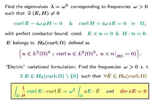
Eigenvalue problem for an homogeneous material
Take \epsilon = 1 and \mu = 1 in the formulation above.
For two-dimensional domains look for solutions of the electric variational problem
(formula in the box of the above image, where curl is the scalar curl of a two-component vector).
Applies to domains 2DomA, 2DomB, 2DomC, 2DomD, 3DomA, 3DomB.
Find first non-zero eigenvalues \lambda .
![]()
Eigenvalue problem for an inhomogeneous material
Applies to the domain 2DomE.
Take \epsilon = \epsilon_1 < 1 for Material 1 and
\epsilon = 1 for Material 2.
Take \mu = 1 in the formulation in the figure above.
Values for \epsilon_1 are proposed, together with computed solutions.
Find first non-zero eigenvalues \lambda .
3. List of solutions
The solutions we provide below are found by a scalar computation, or, sometimes, by an analytic computation. We also give in general an experimental estimate of the number of exact digits: This is the number of digits which remain inchanged under the increase of polynomial approximation degree.
![]()
Maxwell eigenvalues in 2DomA (L-shape)
The Maxwell eigenvalues coincide with the non-zero Neumann eigenvalues.
The solution of the benchmark is computed by a Galerkin approximation of the Neumann eigenvalues with a geometrical refined mesh near the corner (10 layers and ratio 4) and polynomials of "high" degree (degree 10).
0.147562182408E+01
0.353403136678E+01
0.986960440109E+01
0.986960440109E+01
0.113894793979E+02
Note:
The 1rst Maxwell eigenvector has the strong unbounded singularity,
The 2nd one belongs to H^1 ,
The 3rd and 4th one are analytic (exact value of the eigenvalue
\pi^2 = 9.86960440108936)
The 5th one has the strong unbounded singularity.
We expect that at least 11 digits are correct.
![]() Go back to the list of problems
Go back to the list of problems
![]()
Maxwell eigenvalues in 2DomB (Cracked square)
The Maxwell eigenvalues coincide with the non-zero Neumann eigenvalues.
For symmetry reasons, each eigenvector has a determined parity across the internal line [AO] = { x \in [-1 0], y = 0 } which extends the crack line. Those vectors which are even with respect to y coincide with Neumann eigenvectors in the half-square [-1 1] x [0 1] and there eigenvalues are known. Those which are odd are computed by a Galerkin approximation in the half-square with Dirichlet condition on the line [AO] and Neumann conditions everywhere else (geometrical refined mesh near the point O: 10 layers and ratio 4, and polynomials of degree 10).
0.103407400850E+01
0.246740110027E+01
0.404692529140E+01
0.986960440109E+01
0.986960440109E+01
0.108448542781E+02
0.122648958490E+02
0.123370055014E+02
0.197392088022E+02
0.212441074562E+02
Note:
Eigenvalues of rank 2, 4, 5, 8 and 9 correspond to even eigenvectors and are equal to
\pi^2 times 1/4, 1, 1, 5/4 and 2 respectively.
For the remaining ones we expect that at least 9 digits are correct.
![]() Go back to the list of problems
Go back to the list of problems
![]()
Maxwell eigenvalues in 2DomC (Part of a ring)
The Maxwell eigenvalues coincide with the non-zero Neumann eigenvalues.
The solution of the benchmark is computed semi-analytically by the use of the tensor product structure in polar coordinates.
0.255920253252E+01
0.986016708642E+01
0.999151611335E+01
0.127920163189E+02
0.211832931832E+02
The 12 digits are correct.
![]() Go back to the list of problems
Go back to the list of problems
![]()
Maxwell eigenvalues in 2DomD (curved L-shape)
The Maxwell eigenvalues coincide with the non-zero Neumann eigenvalues.
The solution of the benchmark is computed by a Galerkin approximation of the Neumann eigenvalues (non-isoparametric approximation of domain: degree 6, geometrical refined mesh: 10 layers and ratio 4 near the corner, and polynomials of degree 10).
0.181857115231E+01
0.349057623279E+01
0.100656015004E+02
0.101118862307E+02
0.124355372484E+02
We expect that at least 11 digits are correct.
![]() Go back to the list of problems
Go back to the list of problems
![]()
Maxwell eigenvalues in 3DomA (Thick L-shape)
The Maxwell eigenvalues of the tensorized domain 2DomA x [0,1] , are
0.963972384472E+01 (DA1 + NJ0)
Maxwell eigenvalues in 3DomB
(Fichera corner)
No benchmark available until now !! See the results of Maxwell computations.
Maxwell eigenvalues for piecewise constant permittivity in 2DomE
(Square)
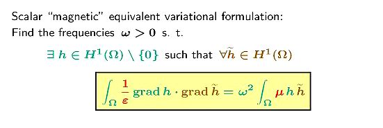
The Maxwell eigenvalues coincide with the non-zero Neumann eigenvalues of the following "magnetic" problem:
According to the description done in Section 2, the permittivity is 1 on a part of the domain, and equal to \epsilon_1 in the other part. In the folllowing tables, we provide eigenvalues of the above scalar problem for the following values of \epsilon_1 :
0.50, 0.10, 0.01, 1E-08.
The solution of the benchmark is computed by a Galerkin approximation of the Neumann eigenvalues with a geometrical refined mesh near the center (10 layers and ratio 4) and polynomials of "high" degree (degree 10).
We indicate in the right column the number of digits which we expect to be correct. It is noticeable that this number strongly depends on the rank of the eigenvalue. This is due to the presence or absence of a strong singularity in (0,0) in the asymptotics of the corresponding eigenvector. We give the value of the minimal singularity exponent \nu of the scalar problem in each case (the Maxwell singularity exponent is then this one minus 1).
Directions to provide feedback. Please give...
Preliminaries
Results
For an easy input in the framework of my web pages, please use the html format. You may take the source of my result page as template (note that it uses the css file core/main.css).
Last modified: 31 August 2004
1. Either the sum of
2. Or the sum of
0.113452262252E+02 (NA1 + DJ1)
0.134036357679E+02 (NA2 + DJ1)
0.151972519265E+02 (DA2 + NJ0)
0.195093282458E+02 (DA1 + NJ1)
0.197392088022E+02 (DA3 + NJ0)
0.197392088022E+02 (NA3 + DJ1)
0.197392088022E+02 (NA4 + DJ1)
0.212590837990E+02 (NA5 + DJ1)
![]() Go back to the list of problems
Go back to the list of problems
![]()
![]()
\epsilon_1 = 0.50
\nu = 0.78365310406121
0.3317548763415E+01
0.3366324157260E+01
0.6186389562488E+01
0.1392632333103E+02
0.1508299096123E+02
0.1577886590819E+02
0.1864329693686E+02
0.2579753111031E+02
0.2985240067684E+02
0.3053785871253E+02
12
12
12
12
12
12
12
12
12
12
\epsilon_1 = 0.10
\nu = 0.38996445808427
0.4533851871670E+01
0.6250332186603E+01
0.7037074196012E+01
0.2234193733540E+02
0.2267919225111E+02
0.2609520456863E+02
0.2650900637498E+02
0.4048783516243E+02
0.4265069898070E+02
0.5588227467094E+02
12
6
12
12
12
8
12
12
12
12
\epsilon_1 = 0.01
\nu = 0.12690206972221
0.4893193324891E+01
0.7206675422492E+01
0.1553698165311E+02
0.2446225024727E+02
0.2448745601340E+02
0.2775724058215E+02
0.2964662366218E+02
0.4424890377211E+02
0.4443521693426E+02
0.6359570343398E+02
12
11
3
12
12
12
3
12
12
11
\epsilon_1 = 1E-08
\nu = 0.00012732395405
0.4934802158785E+01
0.7225211232692E+01
0.2467400464789E+02
0.2467401079360E+02
0.2467401081785E+02
0.2786885061384E+02
0.4441321964155E+02
0.4474562877982E+02
0.6415240830542E+02
0.6415242807291E+02
12
6
8
12
12
7
12
7
8
10
![]() Go back to the list of problems
Go back to the list of problems
![]()
![]()
![]()
A] Your name and affiliation.
B] The name and affiliation of all contributors to computations (including the author(s) of the code).
C] The theoretical principles of your computations
D] The references of the code and a (short) bibliography (papers, preprints, PhD, etc...)
E] Technical data (details on computers, simple or double precision, etc...)
A] The reference of the problem(s) you have solved.
B] The results you found, with preference to a family of results, that is when a parameter is varied (for example, the mesh size, or the approximation degree, or any other approximation parameter). Please provide the values and the relative errors in comparison with the benchmark. Also provide the number of DOF.
![]()