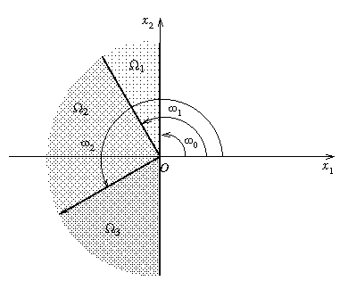
We consider the case of a half-plane where three materials meet as shown on the figure below. We assume there are Dirichlet boudary conditions.
The data file corresponding to the previous configuration is given below. The action chosen is to change the angle2 from
1 to
3 = 270 °.
****** Every line starting with * is ignored.
*      Separate data values with a space or a new line.
*      Maximum length of a data line : 90 characters.
*******************************************************************************
*      Wedge with 3 materials
* Dimension of the space (2 or 3)
2
* Number of domains (K <= 4)
3
* ---> The domains are assumed to be numbered counterclockwise.
* Context for each domain
*   in dimension 2 :
*            1 : isotropic elasticity
*            2 : axisymetric orthotropic elasticity (C11=C22)
*            3 : orthotropic elasticity
*            4 : general elasticity
*   in dimension 3 :
*            1 : isotropic elasticity
*            4 : general elasticity
2 3 2
* Cij coefficients for each domain. According to the context, give
*  in dimension 2 :
*   1 : lambda  mu
*   2 : C11  C12  C66
*   3 : C11  C12  C22  C66
*   4 : C11  C12  C16  C22  C26  C66
*  in dimension 3 :
*   1 : lambda  mu
*   4 : the 21 coefficients in the following order :
*       C11... C16  C22... C26  C33... C36  C44... C46  C55  C56  C66
20.41337 0.91860168 1.1
5. 1. 1. 0.5
1.5384615 0.461538 0.7
* Angles (in degrees) defining the geometry of the domains,
* that is omega(i), i = 0,...K
90 120 180 270
* Boundary conditions at omega(0) and omega(K)
*   1 : Dirichlet
*   2 : Neumann
*   3 : Mixed normal Dirichlet - tangent Neumann
*   4 : Mixed tangent Dirichlet - normal Neumann
*   5 : Transmission
1 1
* Action to be done : integer 10*a1 + a0 such that
* a0 = 0 (Manual computation), 1 (Automatic computation (= AC)),
*      2 (AC + rotation of axes), 3 (AC + variation of the geometry)
*      4 (AC + orientation of the materials), 5 (AC + edge tracking)
*    --> a0 = 2, 4 or 5 in dimension 3 only
* a1 = 0 (Kernel not computed), 1 (Computation of the kernel of A(nu))
*      2 (1 + computation of the singular functions)
3
* Rectangular domain where to search for the roots (necessary if a0 > 0)
* Give  xmin xmax ymin ymax  such that 0 < xmin < xmax and ymin < ymax.
0.1 1.5 -1. 1.
***************** Mutually exclusive specific actions  *****************
* -> Do not modify the keyword "ACTIONi" that marks the beginning of data.
*
ACTION3 (a0 = 3 : Automatic computation + variation of the geometry)
* Variation of the geometry of a domain
* 1) number of the concerned boundary  (0 <= i <= K)
2
* 2) starting angle >=omega(i-1), end angle <= omega(i+1), step (in degrees)
120. 270. 0.5
Running the program with this data file gives the exponents for each position of the internal interface between the materials 2 and 3, given by2 . They are shown on the following figure:
We present here the singular functions corresponding to the exponents computed for2 = 180 ° , where the imaginary part is maximum. This can be easily obtained by modifying slightly the last part of the data file as follows:
The graph of the singular functions are then:
        .
        .
        .
* Action to be done : integer 10*a1 + a0 such that
* a0 = 0 (Manual computation), 1 (Automatic computation (= AC)),
*      2 (AC + rotation of axes), 3 (AC + variation of the geometry)
*      4 (AC + orientation of the materials), 5 (AC + edge tracking)
*    --> a0 = 2, 4 or 5 in dimension 3 only
* a1 = 0 (Kernel not computed), 1 (Computation of the kernel of A(nu))
*      2 (1 + computation of the singular functions)
23
* Rectangular domain where to search for the roots (necessary if a0 > 0)
* Give  xmin xmax ymin ymax  such that 0 < xmin < xmax and ymin < ymax.
0.1 1.5 -1. 1.
***************** Mutually exclusive specific actions  *****************
* -> Do not modify the keyword "ACTIONi" that marks the beginning of data.
*
ACTION3 (a0 = 3 : Automatic computation + variation of the geometry)
* Variation of the geometry of a domain
* 1) number of the concerned boundary  (0 <= i <= K)
2
* 2) starting angle >=omega(i-1), end angle <= omega(i+1), step (in degrees)
180. 180. 0.5
and the stress functions are:
| Summary |