Description

We consider the linear equilibrium equations of an elastic material , possibly heterogeneous: we suppose that can be decomposed in several homogeneous parts _k , with k = 1,. . . ,K. Here we treat corners in two dimensional domains and edges in three dimensional ones. The corners and edges in question are those of , of course, but also those of any of the homogeneous subdomains _k .
The equations in can be written in the general form
L_k u = f    in _k , k=1,. . . ,K, with boundary conditions on and transmission conditions at the interfaces between the _k .

The domain

We denote by d the dimension of the space, d = 2 or 3, and by x_l , l = 1,. . . ,d  the space variables in ^d.

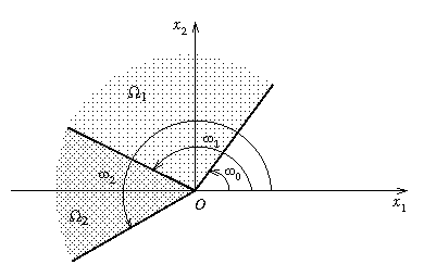
If d = 2, the subdomains _k are polygonal: their boundaries are the union of a finite number of segments whose ends are the corners of . Let  be one those corners. The boundaries in this point define angular sectors lying between the angles _k-1 and _k.
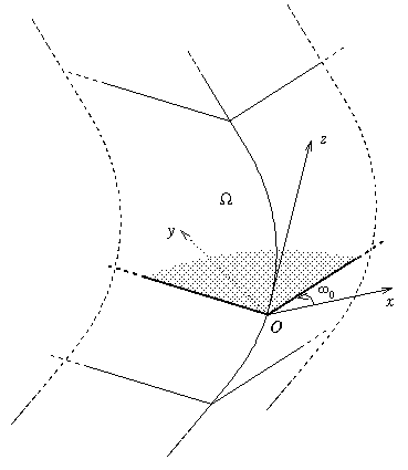
Here follows an example where is made of two domains ₁ and ₂.

If d = 3, we consider domains with edges in the following sense: the boundary of is the union of a finite number of smooth two dimensional surfaces whose boundaries are the edges of . We assume that at each point in an edge of , the domain is locally diffeomorphic to a wedge (a plane sector times ). We cut  by the plane perpendicular to the edge containing and we are reduced to the previous geometry, which allows for the definition of _k.
Here follows an example with one domain.

The system

In one domain , the system L comes from the application of the laws of mechanics in the case of linear elasticity and depends on the classical quantities:

• displacement field u = (u₁, . . .  u_d),
• strain tensor ,
• stress tensor , where a_{i j k l} are elasticity constants satisfying the following symmetry properties a_{i j k l} = a_{j i k l} = a_{i j l k} = a_{k l i j}.

The general equilibrium equation is  L u = f   where   or, taking into account the previous definitions and properties
To simplify the expressions and use the symmetry properties, a common practice is to change the name of the coefficients by setting c_p q = a_{i j k l} . There exists several such numbering conventions ; we are using the following one:

p , q	1	2	3	4	5	6
i j , k l	11	22	33	23	13	12

Each index i , j , k , l varies in {1, . . . d} .

Boundary conditions

Let us define the normal vector n = (n₁, . . . n_d ) at a point on the boundary of the domain. There are essentially two kinds of boundary conditions:

Dirichlet condition	:	u = 0
Neumann condition	:	[(u)] n = 0

In dimension 2, the normal stress T(u) is equal to [(u)] n. In dimension 3, the ``reduced'' normal stress T(u), where the tangential derivative along the edge has to be removed, has to be used.

These conditions have to be set on the two parts of the boundary of the domain, corresponding to the angles ₀ and _K. The conditions can be homogeneous (the same on each part of the boundary) or not. Moreover, we can take into account other types of mixed conditions: we mention normal Dirichlet - tangent Neumann and tangent Dirichlet - normal Neumann.

In dimension 2, we consider the orthonormal basis (n, t ), deduced from (x₁, x₂ ) by a rotation, and we write the boundary conditions in this basis:

• normal Dirichlet - tangent Neumann

1st component	:	u . n = 0
2nd component	:	T(u) . t = 0

• tangent Dirichlet - normal Neumann

1st component	:	u . t = 0
2nd component	:	T(u) . n = 0

In dimension 3, we consider the orthonormal basis (n, t, z), deduced from the local basis (x, y, z) by a rotation around z. The direction z is, by definition, a tangent direction, so we have here one normal direction n and two tangent directions t and z. To the previous components, where x₃ stands for z, we then have to add

Dirichlet tangent	:	u . z = 0
Neumann tangent	:	T(u) . z = 0

A special case is the situation when belongs to the interior of the domain . This means that is an interior transmission point. Then, _K  =  ₀ + 2 and all the domains are filling the space. This situation occur for example in the case of in internal crack.

Singularities

To each corner in two-dimensional domains, and each point of an edge in three-dimensional domains, is associated a family of singular solutions of the elasticity boundary value problems mentioned above, that is to say typical solutions corresponding to non-smooth displacements and stresses, with smooth loadings. These singular solutions have the generic form in polar coordinates ( r, ) centred at :
r f()
where are complex numbers and f are functions of the angular variable.

The are the singularity exponents and take their values in a discrete set depending on the material laws and the openings of the different constitutive parts _k.

The f are piecewise smooth functions: they are smooth in each angular subdomain (_k-1, _k) and are moreover a combination of trigonometric functions.

The aim of this program is the computation of the exponents and the attached functions f  in a region of the complex plane corresponding to the variational regularity, that is a region of the form 0 < Re () < B, with B fixed, in general larger than 1. Practically, the region will be a rectangle because the imaginary part of is, in general, smaller than the real part.

Exponents search method

In the method we are using, the singularity exponents appear as roots of a complex function det(A()) where A() is called the characteristic matrix. To compute those roots, we use Cauchy integrals over closed curves. The user is requested to give a rectangular domain [a, b] × [c, d] in the right half complex plane, where the exponents are to be searched. This rectangle is first split into smaller and smaller rectangles in order to locate the roots. After that, for each root, several approximations are computed until the difference between two successive values is less than a predefined tolerance.
Given a singularity exponent, its opposite and its conjugate are also singularity exponents. So the program computes only the exponents with positive real and imaginary parts. In fact, the exponents are searched with an imaginary part greater than -S_i , where S_i is a small positive number, defined as the separation threshold between real and complex exponents. In order to avoid to get the zero solution when this may occur, the rectangular domain is also limited so that   a > S_r , where S_r is a small positive number.
How to choose the rectangular domain ?
Except when we want to compute an isolated exponent in a ``small'' region, it is better to set c = -d : this symmetry is useful to count the roots at the beginning of the splitting process. The singularity exponents of practical interest have generally a real part lying in the strip [0, 1]. As to the imaginary part, it is usually smaller than 1.
So a first choice for [a, b] × [c, d] can be [0.1, 1.2] × [-1, 1]. The program automatically adjusts this domain if a root is found too close from a boundary of the rectangle by reducing or enlarging the rectangle. Then it starts the search process with the new rectangle.

The results will be obtained faster if the rectangle containing the roots is chosen rather close to the set of roots. A wide range of experiments proves that this choice is generally straightforward and that the first choice settings given above are usually quite satisfactory.